Postgres explain analyze: how to read what the planner picked

seq scan vs index scan, cost units, rows estimate vs actual, BUFFERS, planner statistics, when "Seq Scan" wins

It was a Tuesday when a dashboard query that had run in 80 ms all quarter started taking three seconds. Nothing in the code had changed. I pulled EXPLAIN ANALYZE and the plan had quietly rearranged itself: where it used to build one hash join, it was now running a Nested Loop and probing an index 14,821 times. The planner hadn't broken - it had been handed a bad number and reasoned correctly from it. Everything below is the walk back through that plan, one column at a time, because reading those columns side by side is how we found the single stale statistic behind the whole thing.

When seq scan wins

The first thing I had to rule out that morning was the scan sitting at the bottom of the plan, because a Seq Scan on a big table always looks like the obvious culprit. Sequential scan reads every page in the table from start to finish. Index scan walks the B-tree, then for each match jumps back to the heap to fetch the row. That second jump is random I/O, expensive enough that the planner keeps a knob for it - random_page_cost, default 4.0, against seq_page_cost = 1.0, four times the price per page. Once a query touches a big enough fraction of the rows, reading them in physical order wins outright.

On a small table it isn't even close. A 10,000-row table fits in a handful of pages, and reading all of them is cheaper than even one index lookup with its round-trip overhead. The planner picks Seq Scan here every time, and the index we added just sits there, never chosen.

The fights are usually about low selectivity. We had this exact query flagged as a missing index more than once:

EXPLAIN ANALYZE
SELECT id, email FROM users WHERE active = true;

                                  QUERY PLAN
-----------------------------------------------------------------------------
 Seq Scan on users  (cost=0.00..1834.00 rows=80000 width=36)
                    (actual time=0.012..18.421 rows=80127 loops=1)
   Filter: active
   Rows Removed by Filter: 19873
 Planning Time: 0.142 ms
 Execution Time: 22.110 ms

active = true matches 80% of rows. An index scan there would touch 80,000 random heap pages when one sequential pass reads them all in order, so the planner does the math and stays with Seq Scan. We tried forcing the index once and got a slower plan; the rows actually worth indexing were the rare active = false ones, and a partial index on those is what paid off.

The one that fooled me on that Tuesday was stale statistics, since nothing in the query itself had changed. Postgres keeps row counts and value distributions in pg_stats, and when those drift the cost model drifts with them - the plan looks stupid until you run ANALYZE and it sharpens up again. We covered in Evergreen #4 why vacuum holds the line on disk; ANALYZE is the same daemon's other job, keeping the planner honest, and it's the quiet reason a plan regresses right after a bulk load.

What explain actually reports

Reading my way back to that bad number meant knowing what each node was actually saying, and every node in an EXPLAIN output carries the same shape:

Seq Scan on orders  (cost=0.00..18334.00 rows=1000000 width=72)
                    (actual time=0.014..421.337 rows=998421 loops=1)

cost=A..B is two numbers. A is the startup cost - how much work happens before the first row pops out. For Seq Scan it's basically zero. For a Sort it's the cost of the entire sort, because a sort can't return a row until it has seen all of them. B is the total cost to produce every row the node emits. The unit is arbitrary, calibrated so that reading one sequential page from disk costs 1.0, and everything else gets priced against that single anchor, from per-tuple CPU up to random page reads. I spent a while early on trying to read cost as milliseconds and it never lined up; the wall-clock numbers live in the actual time columns, and cost is only a currency for comparing plans.

rows=N is the planner's estimate of how many rows the node will produce. width=M is the estimated average row size in bytes, which feeds into memory-sizing decisions for sorts and hashes.

The actual time=X..Y rows=N loops=L part is what ANALYZE adds. It re-runs the query (yes, really, it executes it) and records what actually happened. X is the time to first row, Y is total time, both in milliseconds. rows is the truth.

loops is the multiplier you apply by hand to get real numbers. If a node sits inside a Nested Loop and runs once per outer row, loops=5000 means the displayed actual time and rows are per-loop averages. Total wall-clock for that node is actual time × loops, not the number printed. The first time this bit me the plan read 0.02 ms and I believed it - the node had run five thousand times, so the real cost was closer to 100 ms.

Add BUFFERS and you see the I/O directly:

EXPLAIN (ANALYZE, BUFFERS)
SELECT * FROM orders WHERE user_id = 4711;

                                       QUERY PLAN
------------------------------------------------------------------------------------------
 Index Scan using ix_orders_user on orders  (cost=0.42..28.45 rows=12 width=128)
                                            (actual time=0.041..0.082 rows=11 loops=1)
   Index Cond: (user_id = 4711)
   Buffers: shared hit=14
 Planning Time: 0.231 ms
 Execution Time: 0.118 ms

shared hit=14 means 14 buffer-pool pages, all in cache. shared read=14 would mean 14 pages pulled off disk. Cold-cache reads run hundreds of times slower than warm hits, which is why a query that takes 2 ms on your laptop can spike to 600 ms in production right after a restart - same plan, completely different buffer state. The day of the incident, BUFFERS is what told me the slow node was hitting cache, not disk, so I could stop chasing an I/O ghost and look at the row counts instead.

Two more things worth flipping on. VERBOSE shows output columns per node, which matters when you're chasing why a join is carrying a column it doesn't need. SETTINGS dumps any non-default planner GUCs in effect for the query, which catches the case where someone left enable_seqscan = off on a session.

Links

• PostgreSQL docs: EXPLAIN - every option, including BUFFERS, VERBOSE, and SETTINGS.

• PostgreSQL docs: Using EXPLAIN - the canonical walkthrough of the cost, rows, and actual-time columns.

Reading a plan tree

By this point I was reading the plan as a tree, printed depth-first with the root at the top. Each indented child produces rows that its parent consumes, but execution runs the other way: the deepest leaves go first, hand their rows up, and the root finishes last. That backwards order is why I read plans from the bottom, and on that Tuesday the bottom is exactly where the three seconds were hiding.

Hash Join  (cost=312.50..2840.12 rows=1200 width=96)
           (actual time=8.420..142.881 rows=1187 loops=1)
  Hash Cond: (o.user_id = u.id)
  ->  Seq Scan on orders o  (cost=0.00..2210.00 rows=50000 width=72)
                            (actual time=0.011..38.420 rows=49998 loops=1)
  ->  Hash  (cost=200.00..200.00 rows=9000 width=24)
            (actual time=8.120..8.120 rows=9012 loops=1)
        Buckets: 16384  Batches: 1  Memory Usage: 512kB
        ->  Seq Scan on users u  (cost=0.00..200.00 rows=9000 width=24)
                                 (actual time=0.008..3.140 rows=9012 loops=1)

Both Seq Scan nodes run first. users gets hashed into memory. Then orders is streamed past the hash and matched. The join node sits on top, total 142 ms, and the bottleneck is the orders scan, not the join itself.

The join at the top of my plan was the part that had flipped overnight, and there are only three shapes it could have taken. The one I'd been handed was a Nested Loop: it walks one side and probes the other once per outer row, which is brilliant when the outer is tiny - a dozen rows out, ten pulled by index from the inside, a dozen cheap probes and done. The trap is that the planner commits to it on nothing more than its guess about the outer's size. Guess small when the outer is really huge and those dozen probes become a hundred thousand, which is precisely the shape that ate my Tuesday.

What it should have stayed as was a Hash Join - build a hash table on the smaller side, stream the bigger side through it, one pass and out, as long as that smaller side fits in work_mem and the join is on equality. The hash node even tells you whether it fit: Batches of 1 and it stayed in memory, anything higher and it spilled to disk because work_mem was too tight.

That left one shape I almost never saw in our plans. Merge Join zips two already-sorted inputs together, no hash to build and no random I/O, but it only earns its keep when the sort comes for free - usually because both sides arrive straight off index scans on the join keys.

So I went back to the deepest leaf, the way I always do when the costs stop making sense. Joins amplify: that leaf was returning a thousand times the rows the planner expected, and every node above it had inherited the error until the whole plan derailed. Get the bottom node honest and the ones above it usually fall back into line.

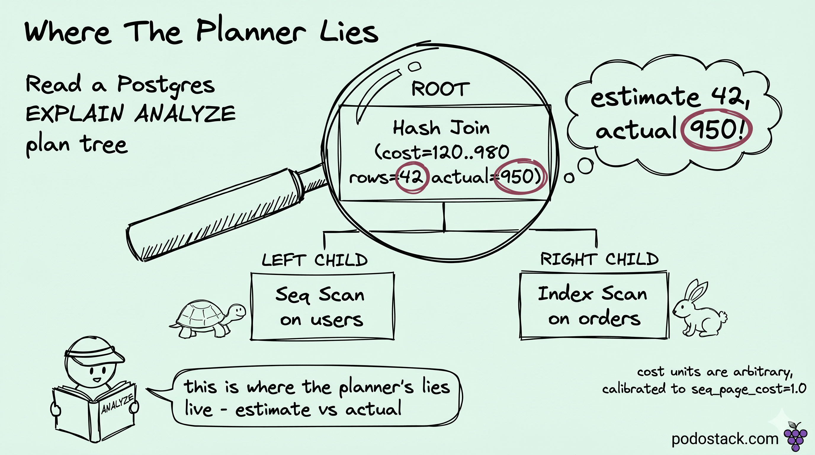
The estimate-vs-actual gap

This is the column that broke my Tuesday, and the one I read first ever since: rows. The planner's estimate against the actual count is the most diagnostic number on the page - a 10x gap makes me look twice, and a 100x gap means the plan was built for a fantasy while the real query runs a completely different shape.

Seq Scan on events  (cost=0.00..18334.00 rows=12 width=72)
                    (actual time=0.014..2840.337 rows=14821 loops=1)
   Filter: ((tenant_id = 4711) AND (kind = 'login'))

Planner thought 12 rows. Reality is 14,821. That gap will pick Nested Loop everywhere because the planner thinks the outer is microscopic, and then probe an index 14,821 times instead of building one hash. Three seconds where it should have been 80 ms.

In our case it was the cause we hit most. An overnight batch job had loaded a few million rows into events, and pg_stats still reflected the pre-load distribution - that's where the estimate of 12 came from. ANALYZE events; snapped it back to something honest, the planner went straight back to a hash join, and the three seconds dropped to 80 ms. Inserts that skip that follow-up ANALYZE are behind most of the "fast yesterday, slow today" tickets we field.

Correlated columns get us more often than I'd like to admit. The planner assumes columns vary independently and multiplies their selectivities, so WHERE country='US' AND state='CA' comes out as 5% × 2% = 0.1%, even though every CA row is already a US row and the honest number is 2%. A 20x under-estimate like that is plenty to drop a Nested Loop on the wrong side; CREATE STATISTICS with dependencies or ndistinct is what teaches the planner that the two columns travel together.

The one that burned a multi-tenant database I worked on was skew. Default stats only keep the top 100 most-common values per column, so a hot tenant sitting just outside that top 100, holding a tenth of the rows, looks like average frequency to the planner. Raising default_statistics_target for the column, or to 500-1000 globally on a big table, widens the histogram until it catches that long tail.

Other times the value the planner needs is hidden behind a function. WHERE lower(email) = 'foo@bar.com' can't touch the stats on email at all, since there's no model for what lower() does to the distribution; you index the expression itself or add extended statistics on it, and the same blind spot turns up with date functions, jsonb extractors, anything that wraps a column.

I look for the lowest node where the rows= estimate misses actual by more than 10x. That's the one feeding bad numbers up the tree, so its statistics get fixed first, then re-plan and see what's still ugly.

Links

• PostgreSQL docs: How the Planner Uses Statistics - where the rows estimate comes from and why it drifts.

• PostgreSQL docs: CREATE STATISTICS - extended statistics for the correlated-columns case.

• PostgreSQL docs: ANALYZE - the command that snaps a stale estimate back to reality.

Tools and shortcuts

After that Tuesday we stopped trusting that we'd be at the keyboard when the next plan flipped. The queries that hurt misbehave when nobody's watching, and you want the plan captured at the moment it goes wrong, not reconstructed from memory the next morning.

auto_explain is the built-in contrib module that logs plans for any query slower than a threshold. Drop this in postgresql.conf:

shared_preload_libraries = 'auto_explain'
auto_explain.log_min_duration = '500ms'
auto_explain.log_analyze = on
auto_explain.log_buffers = on
auto_explain.log_nested_statements = on
auto_explain.log_format = 'json'

Any query past 500 ms gets its full EXPLAIN (ANALYZE, BUFFERS) written to the Postgres log, and JSON is the format the visualisers want. The one caveat: log_analyze = on adds timing overhead per query, usually a few percent. We shipped it anyway - the first cold-cache mystery it explained had already cost us more than the overhead ever would.

Alongside it, pg_stat_statements keeps a running tally per query fingerprint - total time, mean time, rows, buffer hits. The query I reach for first is SELECT * FROM pg_stat_statements ORDER BY total_exec_time DESC LIMIT 20;, because it ranks offenders by total impact rather than by the slowest single call, and that ranking is what tells me which queries are even worth an EXPLAIN. One more line in the config, log_min_duration_statement = 1000, logs the text of anything slower than a second, and paired with auto_explain you get the query and its plan in the same log entry.

When it comes to actually reading a captured plan, I paste it into explain.dalibo.com or explain.depesz.com. Both colour-code the tree by timing, and Dalibo paints the estimate-vs-actual gap red, which is the column I end up staring at first anyway.

Links

• PostgreSQL docs: auto_explain - logging slow-query plans automatically, with log_analyze and log_buffers.

• PostgreSQL docs: pg_stat_statements - aggregate per-query stats for finding what's worth explaining.

• explain.depesz.com and explain.dalibo.com - paste a raw plan, get a colour-coded tree.

Common mistakes

Most of the misreads I still catch come down to trusting a label over the numbers. An index scan isn't automatically faster than a sequential one - on a small table or a wide filter the Seq Scan really is the right call, and forcing the index only slows it down. The cost figures are just the planner's guess, so they tell you less than the gap between estimated and actual rows ever will. And EXPLAIN ANALYZE on a DELETE or UPDATE runs the statement for real, which is why those go inside BEGIN; ... ROLLBACK; for me, or lose the ANALYZE entirely when all I want is the plan.

The rest are habits I had to build the hard way. I keep BUFFERS on, because without it there's no telling warm-cache fast from cold-cache slow, and that's how a buffer-pool problem gets blamed on the query instead. I run ANALYZE after every bulk load now, since fresh data on stale stats is exactly what cost me that Tuesday. A loops count above 1 gets multiplied out before I say anything about a node's time, because that's cardinality and not a bug. And I never fully trust a bare EXPLAIN: the plan it prints is only an intention, and the real numbers can still bend it once ANALYZE actually runs.

Storage was Evergreen #4, the planner was today. Next up is transaction isolation - what READ COMMITTED and REPEATABLE READ actually buy you when two writers collide - and after that JSONB, where it earns its place as a column type and where it quietly becomes a mistake.