Postgres statistics: why the planner picks the wrong index

pg_statistic, ANALYZE, default_statistics_target, extended statistics, autovacuum

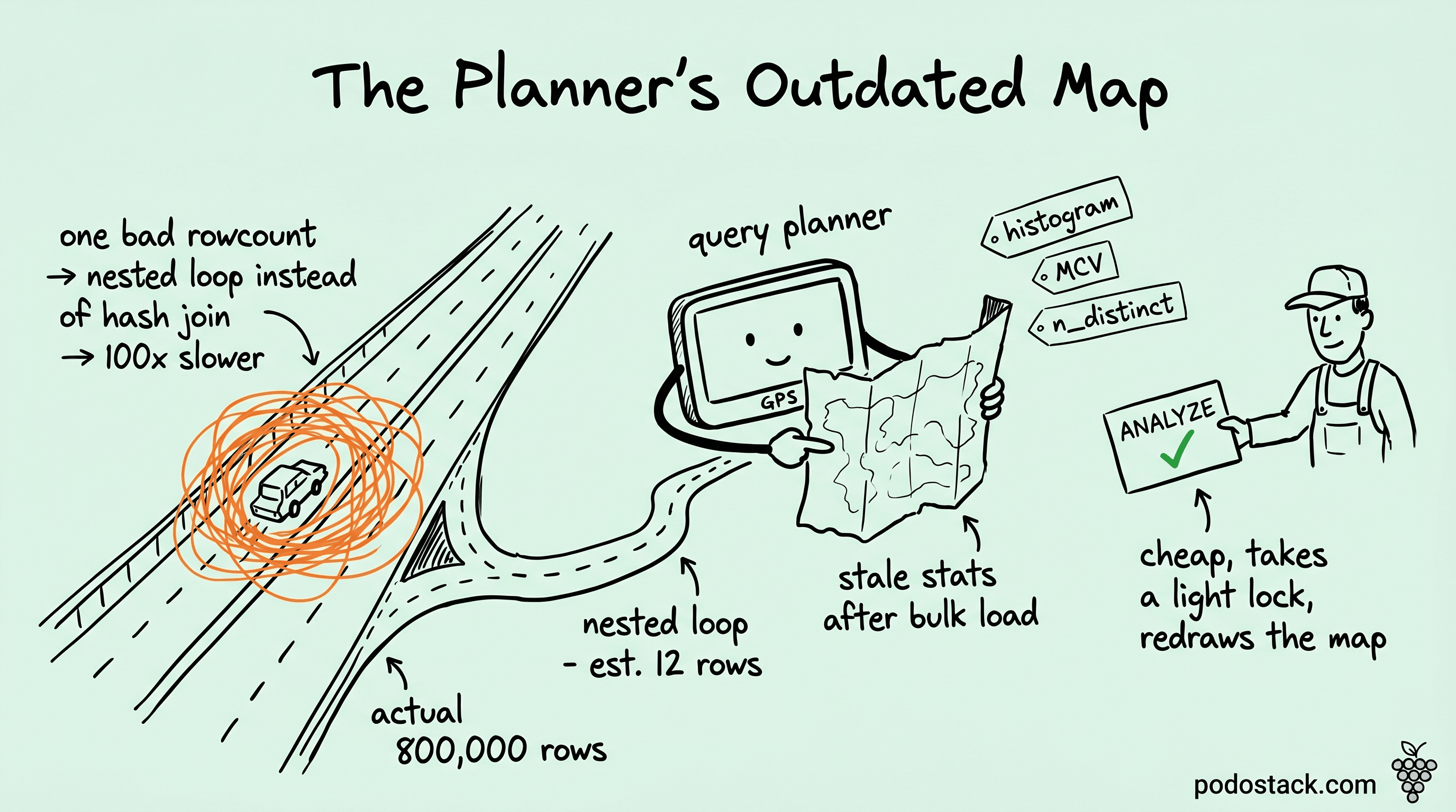
The query had been fast for eight months. A lookup that joined orders to customers, filtered by city and zip, ran in under 10 ms every time, never showed up in pg_stat_statements, nobody thought about it. Then one Tuesday morning the same query started taking nine seconds, and the API behind it started timing out, and the on-call engineer who pulled the plan found a nested loop where there used to be a hash join. Nothing had been deployed. No index had been dropped. What had happened overnight was a 40-million-row bulk import into the orders table, run by a batch job, and that import had quietly invalidated the one thing the planner relies on to make good decisions: its statistics. The query didn't get slower. The planner got dumber, because the numbers it was reasoning from were eight months stale and now described a table that no longer existed.

What the planner is actually reading

Postgres doesn't plan queries by looking at your data. It plans them by looking at a statistical summary of your data, collected by ANALYZE and stored in the pg_statistic catalog. You'll mostly read it through the friendlier pg_stats view, which decodes the internal arrays into something legible. Everything the planner believes about how many rows a filter will return, whether to use an index, which join algorithm to pick - all of it traces back to four pieces of summary kept per column.

The first is n_distinct, an estimate of how many distinct values the column holds. A negative value is a ratio - -1 means every row is unique, -0.5 means roughly half the rows are distinct - which lets the estimate scale as the table grows instead of going stale at a fixed count. The second is the most common values list, most_common_vals, paired with most_common_freqs: the handful of values that appear most often and how frequently each one shows up. This is what lets the planner know that status = 'active' matches 80% of rows while status = 'pending_deletion' matches 0.1%, and treat the two filters completely differently. The third is histogram_bounds, a set of boundary values that divide the rest of the column - everything not already captured in the MCV list - into buckets of roughly equal population, which is how range predicates like created_at > $1 get estimated. The fourth is correlation, a number between -1 and 1 describing how closely the physical order of rows on disk matches the sorted order of the column's values.

That last one quietly decides a lot of index plans, so it's worth dwelling on.

Correlation and the cost of an index scan

Imagine a table where rows were inserted in created_at order and never moved. The on-disk layout almost exactly matches the sort order of created_at, so correlation is near 1.0. When the planner considers an index scan on a range of dates, it knows the matching heap rows are clustered together on a few adjacent pages, so reading them is nearly sequential and cheap. Now imagine a UUID primary key, where the physical position of a row has nothing to do with the value. Correlation is near zero. An index range scan there means the matching rows are scattered across the whole table, one per page in the worst case, and the planner correctly costs that as expensive random I/O - sometimes expensive enough that it picks a sequential scan of the entire table instead, because reading everything in order beats chasing scattered pages.

This is why the same index can be a brilliant choice on one column and one the planner refuses to touch on another, and why a freshly CLUSTER-ed table suddenly gets fast index scans it didn't have before. The correlation figure is doing the talking. When it's wrong - because the stats are stale and the table has been reorganized since the last ANALYZE - the planner costs index scans against a layout that no longer exists.

How statistics go stale, and why bulk loads are the worst case

ANALYZE is what refreshes all of this, and in normal operation you never run it by hand because autovacuum runs it for you. The autovacuum daemon watches how many rows have changed in each table and triggers an analyze when the churn crosses a threshold. The formula is autovacuum_analyze_threshold + autovacuum_analyze_scale_factor * reltuples - a small fixed floor (50 by default) plus a fraction of the table size. The scale factor defaults to 0.1, so on a steady table you get a fresh analyze after about 10% of the rows have been inserted, updated, or deleted. For most workloads this is invisible and fine.

The bulk load is where it breaks, and it breaks in two distinct ways. First, timing: the 40-million-row import dumps all those rows in minutes, but autovacuum doesn't fire mid-transaction, and even after commit there's a delay before the daemon notices and schedules the analyze. In that window - which can be minutes to an hour depending on your autovacuum settings and how busy the daemon is - the planner is working from statistics that describe the table as it was before the import. It thinks the table has the row count it had yesterday, thinks the MCV list still applies, thinks the histogram still covers the real range. Every estimate it makes is anchored to a table that's now a fraction of its current size, and the plans it produces are built on those wrong numbers.

Second, and nastier: if the bulk load is into a brand-new table, or you've just run a migration that rebuilt one, there may be no statistics at all. With nothing in pg_statistic, the planner falls back to hardcoded guesses baked into the source - a fixed assumption that an equality filter matches a small constant fraction of rows, and so on. Those defaults are occasionally close and usually not, and on a large table "usually not" is a sequential scan where an index would have returned in milliseconds.

When one bad estimate cascades

The mechanism that turns one bad number into a hundredfold slowdown is worth tracing, because it's never just one bad estimate sitting there harmlessly. The planner builds a plan bottom-up. It estimates how many rows the filter on orders returns, feeds that estimate into the join above it, and the join algorithm it chooses depends entirely on that row count. If it expects the filter to return 12 rows, a nested loop is the obvious choice - for each of 12 rows, probe the index on customers, done in a flash. If it expects 12 rows and the filter actually returns 800,000 because the stats were stale and the value is far more common than the MCV list claimed, that nested loop now runs 800,000 index probes instead of 12. The plan that was optimal for the estimate is catastrophic for the reality. A hash join, which the planner would have chosen if it had known the true row count, would have read each side once and finished in a fraction of the time.

That's the whole story of the nine-second query. The bulk import made a value far more common than the stale MCV list said it was, the planner underestimated the filter's output by orders of magnitude, picked a nested loop on that underestimate, and the nested loop did hundreds of thousands of times the work it was costed for. The fix was one command - ANALYZE orders - and the query dropped back under 10 ms because the planner could finally see the table it was actually querying. We'd spent twenty minutes reading the query, the index, and the schema, and all three were fine the whole time. What had drifted was the gap between what the planner believed and what was true.

The city/zip trap, and extended statistics

One class of misestimate survives any amount of fresh single-column statistics, and it's the one that bit our opening query. Postgres, by default, assumes columns are statistically independent. When you filter on two columns at once - WHERE city = 'Springfield' AND zip = '62701' - it estimates the combined selectivity by multiplying the two individual selectivities together. If 0.5% of rows are in Springfield and 0.2% have that zip, it concludes that 0.001% of rows match both, multiplying the fractions as if the two facts were unrelated.

But city and zip aren't independent at all. A zip code essentially determines its city - knowing the zip tells you the city for free. The rows matching zip = '62701' are almost entirely a subset of the rows matching city = 'Springfield', so the true combined selectivity is roughly just the zip's selectivity, 0.2%, not the 0.001% the planner computed. The planner underestimates the match count by a couple of hundredfold, and that underestimate feeds straight into the cascade above - it picks a nested loop for what it thinks is a tiny result set, and the result set is two hundred times bigger.

CREATE STATISTICS is the fix, available since Postgres 10. You declare an extended statistics object over the correlated columns and let ANALYZE measure their actual relationship:

CREATE STATISTICS orders_city_zip (dependencies, ndistinct)
  ON city, zip FROM orders;
ANALYZE orders;

The dependencies kind teaches the planner the functional dependency between city and zip, so it stops multiplying their selectivities as if they were independent. The ndistinct kind tracks the number of distinct combinations across the column group, which fixes underestimates in GROUP BY over multiple columns. These extended objects are computed from the same row sample ANALYZE already takes, so they cost almost nothing extra to maintain - but they don't exist until you create them, and Postgres will never create them for you. This is the single most common missing-statistics object in production, and the symptom is always the same: a multi-column filter on related columns that the planner wildly underestimates.

default_statistics_target and when to raise it

The resolution of all this is governed by default_statistics_target, which defaults to 100. That number controls how many entries go in the MCV list and how many buckets the histogram gets - effectively, how detailed a picture ANALYZE paints. For most columns 100 is plenty. For a column with a long, skewed tail of values - where the top 100 most common values don't capture enough of the distribution, and the planner keeps misjudging the less-common ones - raising it helps the estimates a lot.

You can raise it globally, but that's usually the wrong move; it bloats pg_statistic and slows ANALYZE across every column whether they need it or not. The targeted lever is per-column: ALTER TABLE orders ALTER COLUMN customer_id SET STATISTICS 1000. Now that one column gets a 1000-entry MCV list and a finer histogram on the next analyze, and nothing else pays for it. Reach for this when EXPLAIN ANALYZE shows a large gap between estimated and actual rows on a filter against a high-cardinality, skewed column, and the stats are confirmed fresh - raising the target on a column that's simply stale just produces a more detailed wrong answer.

Why ANALYZE is cheap and belongs in every migration

The thing that makes the stale-stats failure so frustrating is how trivial the fix is. ANALYZE reads a sample of the table - not the whole thing, a statistically sufficient sample sized from the statistics target - computes the summaries, and writes them to pg_statistic. On a large table it's seconds, not the minutes a full VACUUM FULL or reindex would take. Crucially, it takes only a light lock. ANALYZE acquires a SHARE UPDATE EXCLUSIVE lock, which lets reads and writes continue against the table the whole time - it does not take the exclusive lock that blocks traffic, so there's no reason to fear running it on a live system during business hours.

Given that, the rule writes itself: any operation that meaningfully changes a table's contents should be followed by an explicit ANALYZE. A bulk import, a large backfill, a migration that rewrites a column, a pg_restore into a fresh database - run ANALYZE on the affected tables before you let production traffic hit them, rather than waiting the minutes-to-an-hour for autovacuum to notice. It costs seconds and it closes exactly the window where the planner is reasoning from a table that no longer exists. The opening incident was nine seconds of timeout per request for the better part of an hour because the batch job didn't end with one cheap command.

The decision framework

When a query that was fine goes sideways, the question is which layer lied, and the order you check matters.

Pull the plan first with EXPLAIN ANALYZE and compare estimated rows against actual rows at each node. A close match all the way up means the planner saw the table correctly and the plan is genuinely the best available - the problem is elsewhere, maybe a missing index or the query itself. A large gap at some node is the planner working from bad numbers, and that gap is where you focus.

If the gap is on a single-column filter, suspect staleness first. Check last_analyze and last_autoanalyze in pg_stat_user_tables, and if they predate a recent bulk change, run ANALYZE and re-check the plan before doing anything more elaborate. If the column is high-cardinality and skewed and the stats are fresh, that's the case for raising its per-column statistics target. If the gap is on a filter spanning two or more related columns - the city/zip shape - no single-column tuning will touch it, and the answer is a CREATE STATISTICS object over the group. If the gap is specifically on index-versus-sequential choice and the table was recently reorganized, look at the correlation figure, which goes stale the same way everything else does.

The ones that page me at 3 AM

Roughly in order of how often each has cost me a night:

• Bulk loading and walking away. The import commits, autovacuum hasn't fired yet, and for the next stretch every plan is built on pre-import statistics. End the load with an explicit ANALYZE and the window never opens.

• Then the independence assumption, where it doesn't hold. City and zip, country and currency, product and category - any pair where one implies the other will be underestimated, sometimes by hundreds of times, until a CREATE STATISTICS object teaches the planner the dependency.

• Raising default_statistics_target globally to fix one column slows every analyze and bloats the catalog for no benefit on the columns that were already fine. Set it per-column where EXPLAIN ANALYZE proves the need.

• Treating a nested-loop blowup as a query problem misses the point. The nested loop wasn't wrong for the row count the planner estimated - the estimate was. Fix the cardinality and the join algorithm fixes itself.

• Fear that ANALYZE will lock the table keeps people from running it, but it takes a SHARE UPDATE EXCLUSIVE lock, reads and writes continue throughout, and it runs in seconds. No reason to schedule it for a maintenance window.

• A restored or freshly-migrated database has no statistics at all, which people forget. Until the first ANALYZE, the planner runs on hardcoded default guesses, which on a large table means sequential scans where indexes existed all along.

• And reading a misestimate without checking last_analyze. Half the "the planner is broken" reports are simply stale statistics, and the check is one query against pg_stat_user_tables before you go hunting for anything subtler.

The planner is only as good as its picture of the data, and that picture is a snapshot that ages. Most of the dramatic, overnight, nothing-changed query regressions you'll chase come down to the snapshot having drifted away from reality - a bulk load that outran autovacuum, a correlated pair the planner was multiplying blind, a restored database nobody analyzed. The catalog tables tell you which one it is, and ANALYZE is almost always the cheapest fix you'll apply all week.