
Star Schema Explained: The Data Pattern Every Engineer Should Know
Fact tables, dimension tables, and why the star schema is still the backbone of data warehousing

A few years ago I joined a company as a backend engineer and was asked to build a dashboard. Simple request - show sales by region, by product category, over time. Classic business intelligence stuff.
I did what any backend engineer would do. I wrote a SQL query joining 11 tables through 6 intermediate junction tables. It took 47 seconds to run. The product manager asked me to add a date filter. The query broke.
A data engineer on the team looked at my query, sighed, and said: “Have you heard of a star schema?”
Two days later I had a schema with 5 tables, queries that ran in under a second, and a dashboard that actually worked. That was my introduction to dimensional modeling, and I’ve never looked at analytics databases the same way since.
What’s wrong with your normal schema?
If you come from application development, you’re used to normalized databases. Third normal form. No data duplication. Foreign keys everywhere. Transactions are consistent. This is great for OLTP - online transaction processing. Your app writes orders, updates inventory, manages user accounts. Normalization keeps the data clean.
But analytics is a different animal. You’re not writing one row at a time. You’re reading millions of rows, aggregating, grouping, filtering across dimensions. Normalized schemas are terrible at this because every query needs to chase foreign keys through a maze of junction tables.
Here’s a typical normalized query for “total sales by product category in Q1”:
-- Normalized: 6 joins, slow, painful
SELECT
    c.category_name,
    SUM(oi.quantity * oi.unit_price) AS total_sales
FROM order_items oi
JOIN orders o ON oi.order_id = o.id
JOIN products p ON oi.product_id = p.id
JOIN product_categories pc ON p.category_id = pc.id
JOIN categories c ON pc.category_id = c.id
JOIN order_dates od ON o.date_id = od.id
WHERE od.quarter = 'Q1'
  AND od.year = 2025
GROUP BY c.category_name;
Six joins. Each join is a lookup. Each lookup is slow at scale. Add a few million orders and this query crawls.
The star schema exists to solve this problem.
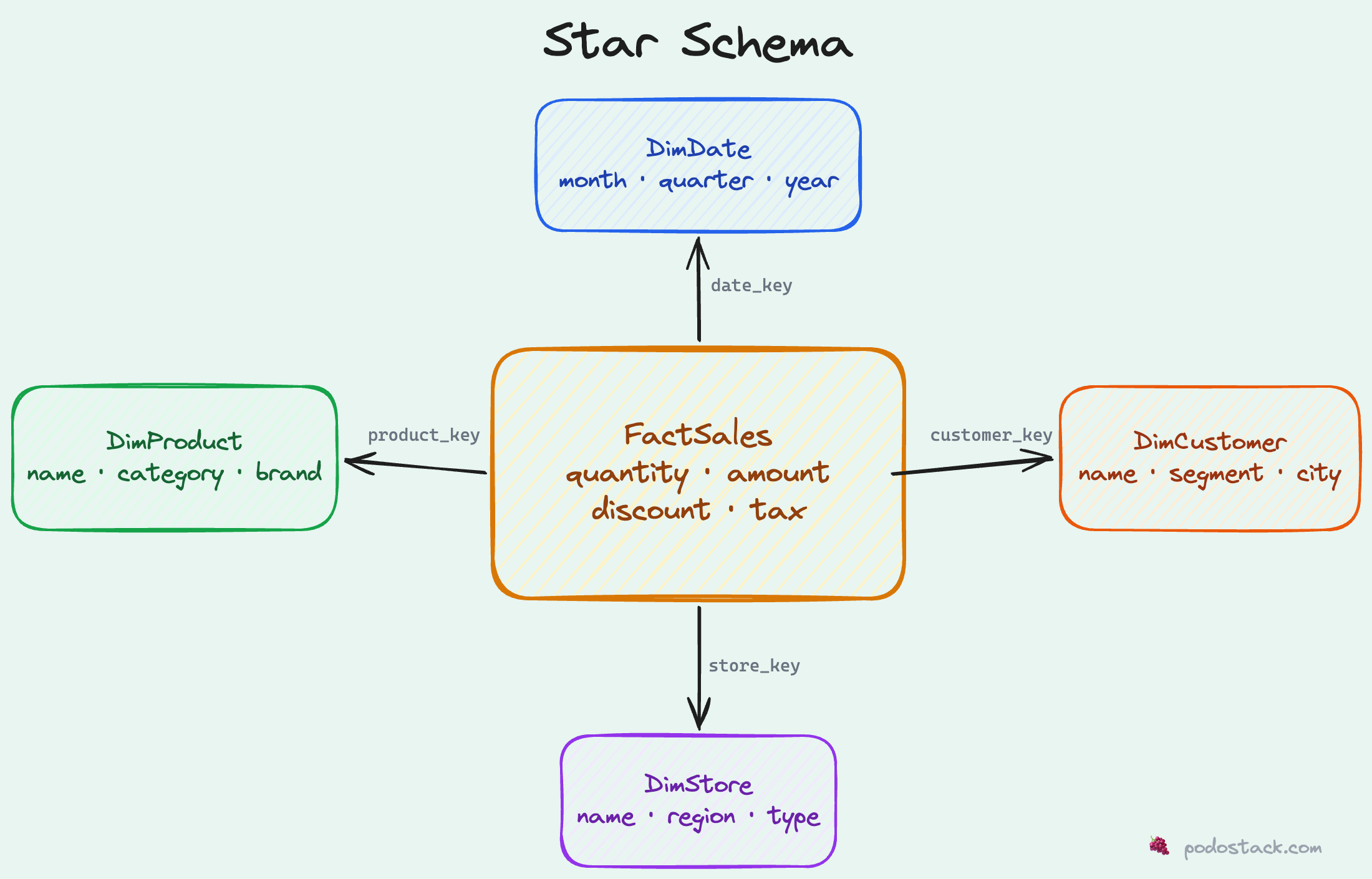
The star schema: center and points
Picture a star. In the center, you have one big table called the fact table. It contains the measurements - the numbers you want to analyze. Sales amounts, quantities, clicks, durations. Things you sum, average, and count.
Radiating outward, you have dimension tables. These describe the context around each measurement. When did it happen? What product? Which customer? What store? Dimensions are the “who, what, where, when” of your data.
The fact table sits in the middle with foreign keys pointing to each dimension. That’s it. That’s the whole pattern. It looks like a star when you draw it, which is where the name comes from.
Let’s build a concrete example.
Building a star schema: e-commerce sales
The fact table
The fact table records events - things that happened. Each row is one transaction, one click, one measurement. It’s typically the biggest table by far.
CREATE TABLE FactSales (
    sale_id       BIGINT PRIMARY KEY,
    date_key      INT NOT NULL,        -- FK to DimDate
    product_key   INT NOT NULL,        -- FK to DimProduct
    customer_key  INT NOT NULL,        -- FK to DimCustomer
    store_key     INT NOT NULL,        -- FK to DimStore
    quantity      INT NOT NULL,
    unit_price    DECIMAL(10,2),
    total_amount  DECIMAL(12,2),
    discount      DECIMAL(10,2),
    tax_amount    DECIMAL(10,2)
);
Notice a few things:
Surrogate keys (
date_key,product_key, etc.) instead of natural keys. More on this later.Numeric measures that you’d aggregate: quantity, amount, discount, tax.
No descriptive text. No product names, no customer emails. That stuff lives in dimensions.
Grain - each row represents one product sold in one transaction. This is crucial. The grain defines what “one row” means in your fact table.
The date dimension
Every analytics schema needs a date dimension. Trust me on this. Even if you think “I’ll just use a date column and date functions,” you’ll regret it when someone asks for “sales in fiscal Q3” or “year-over-year comparison for week 47.”
CREATE TABLE DimDate (
    date_key        INT PRIMARY KEY,      -- e.g., 20250215
    full_date       DATE NOT NULL,
    day_of_week     VARCHAR(10),          -- 'Monday', 'Tuesday'...
    day_of_month    INT,
    month           INT,
    month_name      VARCHAR(10),          -- 'January', 'February'...
    quarter         INT,
    quarter_name    VARCHAR(2),           -- 'Q1', 'Q2'...
    year            INT,
    fiscal_quarter  INT,                  -- If your fiscal year differs
    fiscal_year     INT,
    is_weekend      BOOLEAN,
    is_holiday      BOOLEAN,
    holiday_name    VARCHAR(50)
);
This looks like overkill until you need it. And you will need it. Pre-computing these attributes means your queries don’t need date arithmetic. Filtering by quarter_name = 'Q1' is faster and clearer than EXTRACT(QUARTER FROM date) = 1.
A typical date dimension has one row per day, spanning several years. For a 10-year range, that’s ~3,650 rows. Tiny table. Massive utility.
The product dimension
CREATE TABLE DimProduct (
    product_key     INT PRIMARY KEY,       -- Surrogate key
    product_id      VARCHAR(20),           -- Natural key from source system
    product_name    VARCHAR(200),
    category        VARCHAR(100),
    subcategory     VARCHAR(100),
    brand           VARCHAR(100),
    supplier        VARCHAR(200),
    unit_cost       DECIMAL(10,2),
    is_active       BOOLEAN,
    effective_date  DATE,                  -- For SCD Type 2 (more on this later)
    expiry_date     DATE
);
See the product_key vs product_id distinction? product_id is the natural key from your source system - maybe SKU-12345. product_key is a surrogate integer key generated by your ETL process. Why bother?
Because products change. The name gets updated. The category shifts. The price changes. With surrogate keys, you can keep multiple versions of the same product in your dimension table - each with a different product_key but the same product_id. The fact table points to the version that was current at the time of the sale. This is called a “Slowly Changing Dimension” (SCD Type 2), and it’s how you preserve historical accuracy.
Customer and store dimensions
CREATE TABLE DimCustomer (
    customer_key    INT PRIMARY KEY,
    customer_id     VARCHAR(20),
    first_name      VARCHAR(100),
    last_name       VARCHAR(100),
    email           VARCHAR(200),
    city            VARCHAR(100),
    state           VARCHAR(50),
    country         VARCHAR(50),
    segment         VARCHAR(50),          -- 'Enterprise', 'SMB', 'Consumer'
    signup_date     DATE,
    lifetime_value  DECIMAL(12,2)
);

CREATE TABLE DimStore (
    store_key       INT PRIMARY KEY,
    store_id        VARCHAR(20),
    store_name      VARCHAR(200),
    city            VARCHAR(100),
    state           VARCHAR(50),
    country         VARCHAR(50),
    region          VARCHAR(50),          -- 'Northeast', 'West Coast'
    store_type      VARCHAR(50),          -- 'Retail', 'Online', 'Warehouse'
    open_date       DATE,
    square_footage  INT
);
Notice something? There’s intentional denormalization. The customer’s city, state, and country could be in a separate locations table. In a normalized OLTP database, they would be. But in a star schema, you flatten it. Yes, “New York” is stored a million times across customer rows. That’s fine. The storage cost is negligible compared to the query performance gain of avoiding a join.
Querying the star schema
Now watch what happens to that original 6-join nightmare:
-- Star schema: clean, fast, readable
SELECT
    p.category,
    SUM(f.total_amount) AS total_sales
FROM FactSales f
JOIN DimProduct p ON f.product_key = p.product_key
JOIN DimDate d ON f.date_key = d.date_key
WHERE d.quarter_name = 'Q1'
  AND d.year = 2025
GROUP BY p.category;
Two joins. Clear intent. Runs fast.
Want to add “by region”? One more join:
SELECT
    s.region,
    p.category,
    SUM(f.total_amount) AS total_sales
FROM FactSales f
JOIN DimProduct p ON f.product_key = p.product_key
JOIN DimDate d ON f.date_key = d.date_key
JOIN DimStore s ON f.store_key = s.store_key
WHERE d.quarter_name = 'Q1'
  AND d.year = 2025
GROUP BY s.region, p.category
ORDER BY s.region, total_sales DESC;
Three joins. Still clear. Still fast. Try doing this with 11 normalized tables.
More query patterns
Year-over-year comparison:
SELECT
    d.month_name,
    d.year,
    SUM(f.total_amount) AS monthly_sales
FROM FactSales f
JOIN DimDate d ON f.date_key = d.date_key
WHERE d.year IN (2024, 2025)
GROUP BY d.month_name, d.year, d.month
ORDER BY d.month, d.year;
Top customers by segment:
SELECT
    c.segment,
    c.first_name || ' ' || c.last_name AS customer_name,
    SUM(f.total_amount) AS total_spent,
    COUNT(DISTINCT f.sale_id) AS num_orders
FROM FactSales f
JOIN DimCustomer c ON f.customer_key = c.customer_key
GROUP BY c.segment, customer_name
ORDER BY total_spent DESC
LIMIT 20;
Product performance with time filtering:
SELECT
    p.brand,
    p.category,
    SUM(f.quantity) AS units_sold,
    SUM(f.total_amount) AS revenue,
    AVG(f.discount) AS avg_discount
FROM FactSales f
JOIN DimProduct p ON f.product_key = p.product_key
JOIN DimDate d ON f.date_key = d.date_key
WHERE d.year = 2025
  AND p.is_active = true
GROUP BY p.brand, p.category
HAVING SUM(f.total_amount) > 10000
ORDER BY revenue DESC;
Every query follows the same pattern: start from the fact table, join the dimensions you need, filter, aggregate. Once you internalize this pattern, you can write analytics queries in your sleep.
Beyond e-commerce: SaaS metrics example
Star schemas aren’t just for retail. Here’s how you’d model SaaS subscription metrics:
-- Fact: daily active usage
CREATE TABLE FactDailyUsage (
    usage_id        BIGINT PRIMARY KEY,
    date_key        INT,                 -- FK to DimDate
    account_key     INT,                 -- FK to DimAccount
    feature_key     INT,                 -- FK to DimFeature
    plan_key        INT,                 -- FK to DimPlan
    api_calls       INT,
    active_users    INT,
    storage_mb      DECIMAL(12,2),
    compute_minutes DECIMAL(10,2)
);

-- Dimension: subscription plan
CREATE TABLE DimPlan (
    plan_key        INT PRIMARY KEY,
    plan_name       VARCHAR(50),         -- 'Free', 'Pro', 'Enterprise'
    monthly_price   DECIMAL(10,2),
    max_users INT,
    max_storage_gb INT,
    has_sso BOOLEAN,
    has_audit_log BOOLEAN
);
Same pattern. Different domain. The star schema is domain-agnostic.
Star vs snowflake: when to normalize dimensions
You might hear about the snowflake schema. It’s a star schema where dimensions are further normalized into sub-dimensions:
Star:       FactSales → DimProduct (category, subcategory, brand all in one table)
Snowflake:  FactSales → DimProduct → DimCategory → DimSubcategory
The snowflake saves some storage by deduplicating dimension attributes. But it adds joins. In analytics, joins are the enemy. Every join is latency.
My take: use a star schema unless you have a specific reason not to. The storage overhead of denormalized dimensions is negligible - dimension tables are small compared to fact tables. The query simplicity and performance gain is significant.
The one exception: very large dimension tables (millions of rows) with attributes that change frequently. In that case, normalizing out the volatile attributes into a separate table can make your SCD management simpler. But this is a niche scenario. For 95% of cases, flat dimensions win.
When NOT to use a star schema
Star schemas aren’t universal. Don’t use them for:
OLTP workloads. Your application database should be normalized. Star schemas are optimized for reads, not writes. Inserting a new order into a star schema requires updating multiple tables in coordination. Normalized schemas handle this naturally.
Real-time data. If you need sub-second freshness, a star schema with batch ETL won’t cut it. You’d need a streaming pipeline or a materialized view approach. Though modern tools like dbt and streaming platforms are closing this gap.
Graph-style queries. “Find all customers who bought products that were also bought by customers in segment X” - this kind of traversal is awkward in a star schema. Graph databases handle it better.
Exploratory, schema-on-read workloads. If you don’t know what questions you’ll ask, a data lake with schema-on-read might be more flexible. Star schemas require you to define the grain and dimensions upfront.
Common mistakes
Wrong grain. The grain of your fact table is the most important design decision. “Each row represents one line item in one transaction” is a clear grain. “Each row represents... some sales stuff” is not. If you can’t state the grain in one sentence, stop and rethink.
Too many dimensions on one fact table. If your fact table has 20 foreign keys, something’s off. Most fact tables have 4-8 dimensions. More than that usually means you’re trying to answer too many different questions with one table. Split it into multiple fact tables with different grains.
Skipping the date dimension. “I’ll just use a DATE column.” Famous last words. The first time someone asks for fiscal year grouping, or week-over-week comparison, or “exclude holidays,” you’ll wish you had a proper date dimension.
Not defining surrogate keys. Using natural keys from source systems in your fact table seems simpler. Until that source system changes its key format, or gets replaced, or produces duplicates. Surrogate keys decouple your warehouse from upstream systems. Always use them.
Mixing facts and dimensions. Don’t put descriptive attributes in the fact table. Don’t put measures in dimension tables. The separation is the whole point. If you find yourself querying the fact table for something that isn’t a number you’d aggregate, that attribute belongs in a dimension.
Tools that love star schemas
The star schema isn’t just a theoretical pattern. It’s the assumed data model for a lot of modern tooling:
BI tools (Tableau, Looker, Power BI, Metabase) - all generate optimized SQL against star schemas
Columnar databases (BigQuery, Redshift, Snowflake, ClickHouse) - columnar storage makes star schema aggregations blazing fast
dbt (data build tool) - the de facto standard for defining and testing dimensional models
OLAP engines (Apache Druid, Apache Pinot) - designed specifically for star schema workloads
If you’re using any of these tools, learning the star schema isn’t optional. It’s the foundation everything else is built on.
Getting started
If you want to try this yourself, here’s a minimal setup you can run in any SQL database:
-- Create tables (simplified)
CREATE TABLE DimDate AS
SELECT
    CAST(REPLACE(d::TEXT, '-', '') AS INT) AS date_key,
    d AS full_date,
    EXTRACT(MONTH FROM d) AS month,
    EXTRACT(QUARTER FROM d) AS quarter,
    EXTRACT(YEAR FROM d) AS year
FROM generate_series('2024-01-01'::DATE, '2025-12-31'::DATE, '1 day') AS d;

-- Seed some dimension data, load facts from your source
-- Then start querying with the patterns above
Start with one fact table and three or four dimensions. Get comfortable with the query patterns. Add complexity as your questions get more sophisticated. The star schema scales remarkably well - both in data volume and in schema complexity.